Core Pandas Data Structures
Today we will only focus on the two fundamental structures:
- Series
- DataFrames
The structures we won't have time to explore are Panels, which should be explored when you're ready to do so.
Here are some key ideas behind the data structures provided by Pandas:
- data may be heterogeneous
- when data is numeric, convenience functions exist to provide aggregate statistical operations (
min(),max(),cumsum(),median(),mode(), etc.),
- data structures are decomposable and composable, that is making DataFrames from Series or Series from DataFrame is supported natively,
- data structures are translatable, that is you can create NumPy
NDArray.

Let's play ...
import numpy as np
import pandas as pd
np_ints = np.random.randint(0,51,10)
pd.Series(np_ints)
0    39
1    10
2    29
3    14
4    45
5     2
6    23
7    10
8    41
9     0
dtype: int32
Data in a series do not have to be numeric:
import string
random_letters = [''
                  .join([string.ascii_letters[c] for c in np.random.randint(0,51,10)])
                  for i in range(10)]
pd.Series(random_letters)
0    HmpGnMzKtX
1    PxNgWfPNcT
2    gxOcyftXGJ
3    SndcxpadhV
4    zzJuBAvERU
5    LiqExROQOf
6    nMYLoCcFbp
7    BbFfhmfPsl
8    LuRuNoMkNs
9    csawGHPAIf
dtype: object
We can specify an index if we'd like that will allow us to have meaningful labels to access the data in the Series:
index = ['city', 'state', 'zip', 'neigborhood', 'area_code']
data  = ['Denver', 'CO', '80023', 'Furhman', '303']
s = pd.Series(data, index)
s
city            Denver
state               CO
zip              80023
neigborhood    Furhman
area_code          303
dtype: object
Now we can access the data by its index label ...
s['city'], s['state']
('Denver', 'CO')
Accessing data in a series is much like accessing data in a Python list. The usual slicing operator is available to get at the data in the Series.
s[1]
'CO'
s[0:3]
city     Denver
state        CO
zip       80023
dtype: object
s[0:3:2]
city    Denver
zip      80023
dtype: object
More sophisticated slicing by index using integers can be achieved with iloc. Here are some simple examples:
s.iloc[0:3]
city     Denver
state        CO
zip       80023
dtype: object
s.iloc[0:3:2]
city    Denver
zip      80023
dtype: object
We can pass a list of the indices we'd like just as easily ...
s.iloc[[1,2,4]]
state           CO
zip          80023
area_code      303
dtype: object
To get at all the values of the Series as an NDArray, simply do
s.values
array(['Denver', 'CO', '80023', 'Furhman', '303'], dtype=object)
which then allows us to convert to a list
s.values.tolist()
['Denver', 'CO', '80023', 'Furhman', '303']
DataFrames
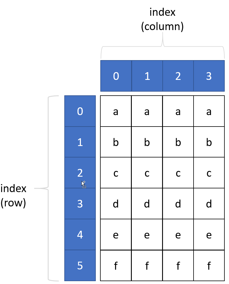
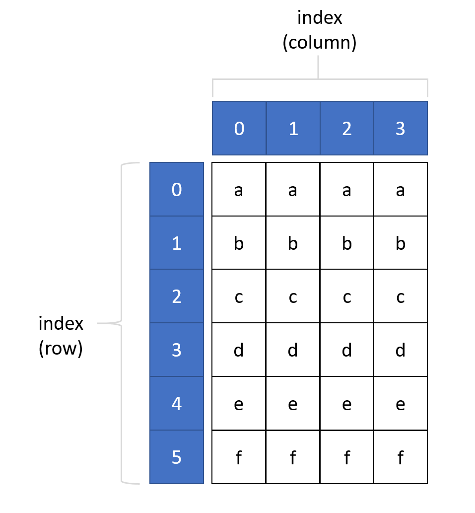
DataFrames are a natural extension to Series in that they are 2-dimensional, and similarly to matrices (from vectors). They have many of the same operations (extended to 2 dimensions), but have some additional properties and operations.

We'll cover the basics here:
- a DataFrame has a row and column axis, which defaults to numeric values (0 and 1),
- a DataFrame axis can be multi-level, that is multi-level indices can be created for row, column or both,
- DataFrames can be converted to
NDArrayand thus be converted to lists and dictionaries, - indexing is achieved either by integer value or index label (both where applicable),
- DataFrame values may be heterogeous.
Let's first begin by building a DataFrame from a 2D Numpy array ...
df = pd.DataFrame(np.random.randint(1,100,100).reshape(10,10))
df
| 0 | 1 | 2 | 3 | 4 | 5 | 6 | 7 | 8 | 9 | |
|---|---|---|---|---|---|---|---|---|---|---|
| 0 | 2 | 38 | 48 | 35 | 13 | 74 | 22 | 39 | 81 | 8 |
| 1 | 78 | 86 | 78 | 11 | 79 | 86 | 81 | 34 | 67 | 94 |
| 2 | 16 | 92 | 41 | 44 | 61 | 40 | 29 | 58 | 94 | 68 |
| 3 | 35 | 87 | 18 | 48 | 48 | 36 | 31 | 65 | 4 | 11 |
| 4 | 63 | 4 | 32 | 59 | 93 | 62 | 48 | 97 | 30 | 76 |
| 5 | 94 | 6 | 90 | 40 | 90 | 32 | 57 | 87 | 47 | 87 |
| 6 | 48 | 64 | 77 | 63 | 18 | 53 | 70 | 4 | 17 | 18 |
| 7 | 92 | 90 | 75 | 22 | 64 | 2 | 19 | 28 | 26 | 2 |
| 8 | 91 | 5 | 60 | 95 | 42 | 47 | 69 | 88 | 33 | 60 |
| 9 | 76 | 7 | 78 | 49 | 92 | 64 | 98 | 43 | 48 | 25 |
[] operator for basic slicing
- the slicing operator
[]works on DataFrames over row slices.
- this operator sparingly it is not consistent with
locandiloc, and may create confusing code if mixed arbitrarily with those selectors
df[1:4] # selecting the rows index 1 to 4
| 0 | 1 | 2 | 3 | 4 | 5 | 6 | 7 | 8 | 9 | |
|---|---|---|---|---|---|---|---|---|---|---|
| 1 | 78 | 86 | 78 | 11 | 79 | 86 | 81 | 34 | 67 | 94 |
| 2 | 16 | 92 | 41 | 44 | 61 | 40 | 29 | 58 | 94 | 68 |
| 3 | 35 | 87 | 18 | 48 | 48 | 36 | 31 | 65 | 4 | 11 |
df[0:4][1] # selecting rows index 0 to 4, column index 1
0    38
1    86
2    92
3    87
Name: 1, dtype: int32
df[1] # selecting column 1, rows 0 .. n
0    38
1    86
2    92
3    87
4     4
5     6
6    64
7    90
8     5
9     7
Name: 1, dtype: int32
df[1][4] # selecting the value at row index 4, column index 1
4
iloc[]
ilocis an integer-based selector. As such, you will need to know the integer values of the row or column indices as necessary
- you may see some correspondence with the
[]selector, but it provides much more
df.iloc[1] # row index 1, returns the full ROW
0    78
1    86
2    78
3    11
4    79
5    86
6    81
7    34
8    67
9    94
Name: 1, dtype: int32
df.iloc[1,2] # row index 1, column index 2
78
df.iloc[1,:] # row index 1, as above
0    78
1    86
2    78
3    11
4    79
5    86
6    81
7    34
8    67
9    94
Name: 1, dtype: int32
df.iloc[1,2:4] # row index 2, column index 2:3
2    78
3    11
Name: 1, dtype: int32
df.iloc[1:2,:] # row index 1:2, column index 0:-1 same as above
| 0 | 1 | 2 | 3 | 4 | 5 | 6 | 7 | 8 | 9 | |
|---|---|---|---|---|---|---|---|---|---|---|
| 1 | 78 | 86 | 78 | 11 | 79 | 86 | 81 | 34 | 67 | 94 |
More sophisticated slicing
More sophisticated slicing can be done over integer indices. For example, if we wanted specific rows and columns for slicing.
Just remember,
- the first argument to the selector is the row
- and the second, the column
df.iloc[1:2,2:5] # row index 1:2, column index 2:5
| 2 | 3 | 4 | |
|---|---|---|---|
| 1 | 78 | 11 | 79 |
df.iloc[[1,3,7], [2,5,6]] # row indices 1,3,7 column indices 2,5,6
| 2 | 5 | 6 | |
|---|---|---|---|
| 1 | 78 | 86 | 81 |
| 3 | 18 | 36 | 31 |
| 7 | 75 | 2 | 19 |
loc()
loc() is a label-based selector, and provides a much richer experience in selecting data.
- it improves the overall readibility of analysis code and also
- it allows for multi-indices to become more easily understood
df_si = pd.DataFrame(df.values,
                     index=['r{}'.format(i) for i in range(0,10)],
                     columns=['c{}'.format(i) for i in range(0,10)])
df_si
| c0 | c1 | c2 | c3 | c4 | c5 | c6 | c7 | c8 | c9 | |
|---|---|---|---|---|---|---|---|---|---|---|
| r0 | 2 | 38 | 48 | 35 | 13 | 74 | 22 | 39 | 81 | 8 |
| r1 | 78 | 86 | 78 | 11 | 79 | 86 | 81 | 34 | 67 | 94 |
| r2 | 16 | 92 | 41 | 44 | 61 | 40 | 29 | 58 | 94 | 68 |
| r3 | 35 | 87 | 18 | 48 | 48 | 36 | 31 | 65 | 4 | 11 |
| r4 | 63 | 4 | 32 | 59 | 93 | 62 | 48 | 97 | 30 | 76 |
| r5 | 94 | 6 | 90 | 40 | 90 | 32 | 57 | 87 | 47 | 87 |
| r6 | 48 | 64 | 77 | 63 | 18 | 53 | 70 | 4 | 17 | 18 |
| r7 | 92 | 90 | 75 | 22 | 64 | 2 | 19 | 28 | 26 | 2 |
| r8 | 91 | 5 | 60 | 95 | 42 | 47 | 69 | 88 | 33 | 60 |
| r9 | 76 | 7 | 78 | 49 | 92 | 64 | 98 | 43 | 48 | 25 |
Selecting contiguous slices (indices are sorted), is very straightforward.
df_si.loc['r3':'r4',]
| c0 | c1 | c2 | c3 | c4 | c5 | c6 | c7 | c8 | c9 | |
|---|---|---|---|---|---|---|---|---|---|---|
| r3 | 35 | 87 | 18 | 48 | 48 | 36 | 31 | 65 | 4 | 11 |
| r4 | 63 | 4 | 32 | 59 | 93 | 62 | 48 | 97 | 30 | 76 |
As expected we can slice the columns as well.
df_si.loc['r3':'r4', 'c2':'c3']
| c2 | c3 | |
|---|---|---|
| r3 | 18 | 48 |
| r4 | 32 | 59 |
... on to Part II: Importing Data.